GDP components over time and among countries
At the risk of oversimplifying things, the main components of gross domestic product, GDP are personal consumption (C), business investment (I), government spending (G) and net exports (exports - imports). There are more about GDP and the different approaches in calculating at the Wikipedia GDP page.
The GDP data we will look at is from the United Nations’ National Accounts Main Aggregates Database, which contains estimates of total GDP and its components for all countries from 1970 to today. We will look at how GDP and its components have changed over time, and compare different countries and how much each component contributes to that country’s GDP.
UN_GDP_data  <-  read_excel(here::here("data", "Download-GDPconstant-USD-countries.xls"), # Excel filename
                sheet="Download-GDPconstant-USD-countr", # Sheet name
                skip=2) # Number of rows to skip
The first thing we will do is to tidy the data, as it is in wide format and we will make it into long, tidy format. We will express all figures in billions rename the indicators into shorter names.
long_UN_Gdp_data<- pivot_longer(UN_GDP_data,cols=4:51,names_to="year",values_to="Spending") #changing it to long format

#Converting
long_UN_Gdp_data$Spending<-as.numeric(long_UN_Gdp_data$Spending)/(10^9)
long_UN_Gdp_data$year<-as.numeric(long_UN_Gdp_data$year)

skimr::skim(long_UN_Gdp_data)| Name | long_UN_Gdp_data |
| Number of rows | 176880 |
| Number of columns | 5 |
| _______________________ | |
| Column type frequency: | |
| character | 2 |
| numeric | 3 |
| ________________________ | |
| Group variables | None |
Variable type: character
| skim_variable | n_missing | complete_rate | min | max | empty | n_unique | whitespace |
|---|---|---|---|---|---|---|---|
| Country | 0 | 1 | 4 | 34 | 0 | 220 | 0 |
| IndicatorName | 0 | 1 | 17 | 88 | 0 | 17 | 0 |
Variable type: numeric
| skim_variable | n_missing | complete_rate | mean | sd | p0 | p25 | p50 | p75 | p100 | hist |
|---|---|---|---|---|---|---|---|---|---|---|
| CountryID | 0 | 1.00 | 439.2 | 254.1 | 4 | 214.00 | 440.0 | 660.0 | 894 | ▇▇▇▇▆ |
| year | 0 | 1.00 | 1993.5 | 13.8 | 1970 | 1981.75 | 1993.5 | 2005.2 | 2017 | ▇▇▇▇▇ |
| Spending | 15421 | 0.91 | 72.2 | 447.4 | -568 | 0.36 | 2.5 | 17.9 | 17349 | ▇▁▁▁▁ |
long_UN_Gdp_data$IndicatorName<-factor(long_UN_Gdp_data$IndicatorName)
summary(long_UN_Gdp_data$IndicatorName)
## Agriculture, hunting, forestry, fishing (ISIC A-B)
## 10464
## Changes in inventories
## 8448
## Construction (ISIC F)
## 10560
## Exports of goods and services
## 10512
## Final consumption expenditure
## 10560
## General government final consumption expenditure
## 10512
## Gross capital formation
## 10512
## Gross Domestic Product (GDP)
## 10560
## Gross fixed capital formation (including Acquisitions less disposals of valuables)
## 10512
## Household consumption expenditure (including Non-profit institutions serving households)
## 10512
## Imports of goods and services
## 10464
## Manufacturing (ISIC D)
## 10560
## Mining, Manufacturing, Utilities (ISIC C-E)
## 10560
## Other Activities (ISIC J-P)
## 10560
## Total Value Added
## 10560
## Transport, storage and communication (ISIC I)
## 10512
## Wholesale, retail trade, restaurants and hotels (ISIC G-H)
## 10512tidy_GDP_data<-long_UN_Gdp_data %>%
mutate(
IndicatorName = case_when(
IndicatorName == "Agriculture, hunting, forestry, fishing (ISIC A-B)" ~ "AHFF",
IndicatorName == "Changes in inventories " ~ "Inventory",
IndicatorName == "Construction (ISIC F)" ~ "Construction",
IndicatorName == "Final consumption expenditure" ~ "Consumption",
IndicatorName == "Exports of goods and services" ~ "Exports",
IndicatorName == "General government final consumption expenditure" ~ "Government_expenditure",
IndicatorName == "Gross capital formation" ~ "Gross_Capital_Formation",
IndicatorName == "Gross Domestic Product (GDP)" ~ "GDP",
IndicatorName == "Gross fixed capital formation (including Acquisitions less disposals of valuables)" ~ "Fixed Capital",
IndicatorName == "Household consumption expenditure (including Non-profit institutions serving households)" ~ "Household_expenditure",
IndicatorName == "Imports of goods and services" ~ "Imports",
IndicatorName == "Manufacturing (ISIC D)" ~ "Manufacturing",
IndicatorName == "Mining, Manufacturing, Utilities (ISIC C-E)" ~ "MMU",
IndicatorName == "Other Activities (ISIC J-P)" ~ "Other",
IndicatorName == "Total Value Added" ~ "Total Value Added",
IndicatorName == "Transport, storage and communication (ISIC I)" ~ "Transport",
IndicatorName == "Wholesale, retail trade, restaurants and hotels (ISIC G-H)" ~ "Retail"
))
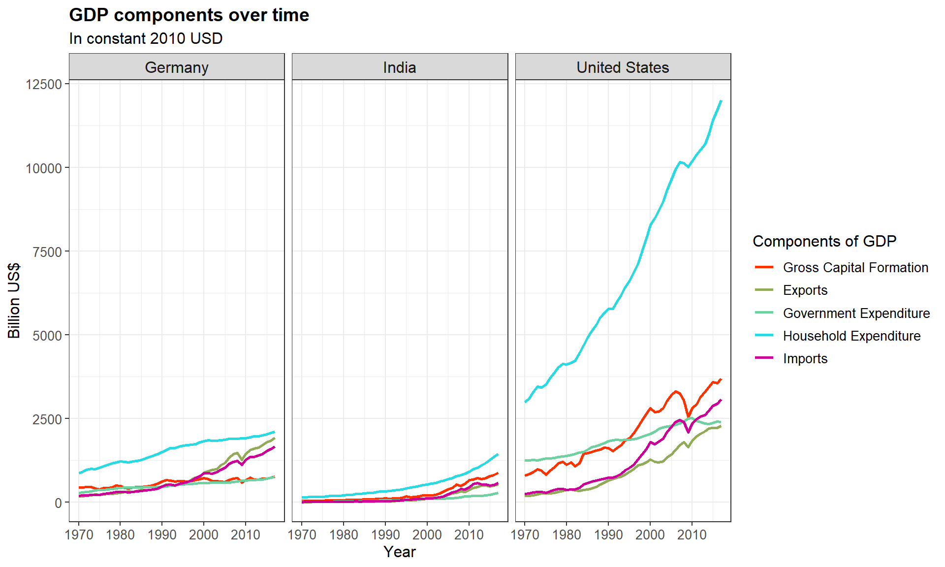
# Let us compare GDP components for these 3 countries
country_list <- c("United States","India", "Germany")GDP Breakdown for Germany, India and United States
tidy_GDP_data %>%
  filter(Country %in% country_list,
         IndicatorName %in% c("Gross_Capital_Formation",
                          "Exports",
                          "Government_expenditure",
                          "Household_expenditure",
                          "Imports")) %>%
  mutate(
    IndicatorName = factor(IndicatorName,
                           ordered=TRUE,
                           levels=c("Gross_Capital_Formation",
                                    "Exports",
                                    "Government_expenditure",
                                    "Household_expenditure",
                                    "Imports"),
                           labels = c("Gross Capital Formation",
                                      "Exports",
                                      "Government Expenditure",
                                      "Household Expenditure",
                                      "Imports"))
  ) %>%
  ggplot(aes(x=year,
             y=Spending,
             colour=IndicatorName,
             group = IndicatorName))+
  geom_line(size = 1)+
  facet_wrap(~Country)+
  labs(title="GDP components over time",
       x="Year",y="Billion US$",
       subtitle="In constant 2010 USD",
       colour="Components of GDP")+
  theme_bw()+
  scale_color_manual(values=c("#FF3300", "#92ab59", "#6fd1a0", "#29dae3",
                             "#CC0099"))+
  theme(
    plot.title = element_text(size = 14, face="bold"),
    plot.subtitle = element_text(size = 12),
    axis.title.x = element_text(size = 12),
    axis.title.y = element_text(size = 12),
    strip.text = element_text(size = 12),
    axis.text.x = element_text(size = 10),
    axis.text.y = element_text(size = 10),
    legend.title = element_text(size = 12),
    legend.text = element_text(size = 10)
  )
Secondly, given that GDP is the sum of Household Expenditure (Consumption C), Gross Capital Formation (business investment I), Government Expenditure (G) and Net Exports (exports - imports). Even though there is an indicator Gross Domestic Product (GDP) in our dataframe, We will calculate it given its components discussed above.
wide_format_gdp<- tidy_GDP_data %>%
  pivot_wider(names_from= IndicatorName, values_from= Spending) %>%
  select(Country,
         year,
         Gross_Capital_Formation,
         Exports, Imports,
         Household_expenditure,
         Government_expenditure,GDP) %>%
  filter(Country %in% country_list) %>%
  group_by(year) %>%
  mutate(Net_Exports=Exports-Imports,
         GDP_calculated=Gross_Capital_Formation+Household_expenditure+
           Government_expenditure+Net_Exports,
         percentage_difference=((GDP_calculated-GDP)/GDP)*100)

wide_format_gdp %>%
  select(Country, year, GDP, GDP_calculated, percentage_difference)
## # A tibble: 144 x 5
## # Groups: year [48]
## Country year GDP GDP_calculated percentage_difference
## <chr> <dbl> <dbl> <dbl> <dbl>
## 1 Germany 1970 1534. 1581. 3.03
## 2 Germany 1971 1582. 1638. 3.54
## 3 Germany 1972 1650. 1709. 3.56
## 4 Germany 1973 1729. 1779. 2.92
## 5 Germany 1974 1744. 1775. 1.78
## 6 Germany 1975 1729. 1780. 2.93
## 7 Germany 1976 1815. 1866. 2.83
## 8 Germany 1977 1876. 1927. 2.77
## 9 Germany 1978 1932. 1991. 3.05
## 10 Germany 1979 2012. 2081. 3.44
## # ... with 134 more rowsThe self-calculated GDP is generally higher compared to the GDP provided in the dataframe by a few percentage points. However, there are also a few years in which the calculated GDP is lower than the provided GDP. Consequently, we can see that there is some deviation between self-calculated GDPs and provided GDPs.
In the chart above, we can see the percentage of GDP which is spent on each of the four main GDP components, across Germany, India and the US. It is evident that for all three countries the biggest component is that of ‘Household expenditure’ with about 60% of GDP comprising of it. For India, Household expenditure proportion has significantly decreased over time from about 70% to 55% today. This does not necessarily mean India’s Household expenditure is decreasing in absolute value. In turn, there has been a large increase in ‘Gross capital formation’ from 20% to about 35%. As India is an emerging economy, this is telling us that India has increased investment in capital good unproportionally over the years. The more capital a country possesses the more potential it has to grow in the long term.
The distribution across GDP components for Germany and the US is similar. This is no surprise since both countries are more developed than India. One major difference across these two countries is the fact that the US has been experiencing a slight increase in the percentage of GDP in household spending of about 5% and has a trade deficit over the years that is as low as 5%. Whereas for Germany where Household spending seems to slightly decrease, net exports have increased from having a trade deficit a few decades ago to a surplus of about 8%.
Generally, for developed countries in the long term, the proportions of all four components of GDP should see less variability than the proportions for emerging countries. This is exactly what is shown by the comparison between developed countries (Germany, US) and emerging economy (India).