IBM HR Analytics

For this task, you will analyse a data set on Human Resource Analytics. The IBM HR Analytics Employee Attrition & Performance data set is a fictional data set created by IBM data scientists. Among other things, the data set includes employees’ income, their distance from work, their position in the company, their level of education, etc. A full description can be found on the website.
First let us load the data
hr_dataset <- read_csv(file = ("D:/r_excluded/my_website/data/datasets_1067_1925_WA_Fn-UseC_-HR-Employee-Attrition.csv"))
glimpse(hr_dataset)
## Rows: 1,470
## Columns: 35
## $ Age <dbl> 41, 49, 37, 33, 27, 32, 59, 30, 38, 36, 35, 2~
## $ Attrition <chr> "Yes", "No", "Yes", "No", "No", "No", "No", "~
## $ BusinessTravel <chr> "Travel_Rarely", "Travel_Frequently", "Travel~
## $ DailyRate <dbl> 1102, 279, 1373, 1392, 591, 1005, 1324, 1358,~
## $ Department <chr> "Sales", "Research & Development", "Research ~
## $ DistanceFromHome <dbl> 1, 8, 2, 3, 2, 2, 3, 24, 23, 27, 16, 15, 26, ~
## $ Education <dbl> 2, 1, 2, 4, 1, 2, 3, 1, 3, 3, 3, 2, 1, 2, 3, ~
## $ EducationField <chr> "Life Sciences", "Life Sciences", "Other", "L~
## $ EmployeeCount <dbl> 1, 1, 1, 1, 1, 1, 1, 1, 1, 1, 1, 1, 1, 1, 1, ~
## $ EmployeeNumber <dbl> 1, 2, 4, 5, 7, 8, 10, 11, 12, 13, 14, 15, 16,~
## $ EnvironmentSatisfaction <dbl> 2, 3, 4, 4, 1, 4, 3, 4, 4, 3, 1, 4, 1, 2, 3, ~
## $ Gender <chr> "Female", "Male", "Male", "Female", "Male", "~
## $ HourlyRate <dbl> 94, 61, 92, 56, 40, 79, 81, 67, 44, 94, 84, 4~
## $ JobInvolvement <dbl> 3, 2, 2, 3, 3, 3, 4, 3, 2, 3, 4, 2, 3, 3, 2, ~
## $ JobLevel <dbl> 2, 2, 1, 1, 1, 1, 1, 1, 3, 2, 1, 2, 1, 1, 1, ~
## $ JobRole <chr> "Sales Executive", "Research Scientist", "Lab~
## $ JobSatisfaction <dbl> 4, 2, 3, 3, 2, 4, 1, 3, 3, 3, 2, 3, 3, 4, 3, ~
## $ MaritalStatus <chr> "Single", "Married", "Single", "Married", "Ma~
## $ MonthlyIncome <dbl> 5993, 5130, 2090, 2909, 3468, 3068, 2670, 269~
## $ MonthlyRate <dbl> 19479, 24907, 2396, 23159, 16632, 11864, 9964~
## $ NumCompaniesWorked <dbl> 8, 1, 6, 1, 9, 0, 4, 1, 0, 6, 0, 0, 1, 0, 5, ~
## $ Over18 <chr> "Y", "Y", "Y", "Y", "Y", "Y", "Y", "Y", "Y", ~
## $ OverTime <chr> "Yes", "No", "Yes", "Yes", "No", "No", "Yes",~
## $ PercentSalaryHike <dbl> 11, 23, 15, 11, 12, 13, 20, 22, 21, 13, 13, 1~
## $ PerformanceRating <dbl> 3, 4, 3, 3, 3, 3, 4, 4, 4, 3, 3, 3, 3, 3, 3, ~
## $ RelationshipSatisfaction <dbl> 1, 4, 2, 3, 4, 3, 1, 2, 2, 2, 3, 4, 4, 3, 2, ~
## $ StandardHours <dbl> 80, 80, 80, 80, 80, 80, 80, 80, 80, 80, 80, 8~
## $ StockOptionLevel <dbl> 0, 1, 0, 0, 1, 0, 3, 1, 0, 2, 1, 0, 1, 1, 0, ~
## $ TotalWorkingYears <dbl> 8, 10, 7, 8, 6, 8, 12, 1, 10, 17, 6, 10, 5, 3~
## $ TrainingTimesLastYear <dbl> 0, 3, 3, 3, 3, 2, 3, 2, 2, 3, 5, 3, 1, 2, 4, ~
## $ WorkLifeBalance <dbl> 1, 3, 3, 3, 3, 2, 2, 3, 3, 2, 3, 3, 2, 3, 3, ~
## $ YearsAtCompany <dbl> 6, 10, 0, 8, 2, 7, 1, 1, 9, 7, 5, 9, 5, 2, 4,~
## $ YearsInCurrentRole <dbl> 4, 7, 0, 7, 2, 7, 0, 0, 7, 7, 4, 5, 2, 2, 2, ~
## $ YearsSinceLastPromotion <dbl> 0, 1, 0, 3, 2, 3, 0, 0, 1, 7, 0, 0, 4, 1, 0, ~
## $ YearsWithCurrManager <dbl> 5, 7, 0, 0, 2, 6, 0, 0, 8, 7, 3, 8, 3, 2, 3, ~I am going to clean the data set, as variable names are in capital letters, some variables are not really necessary, and some variables, e.g., education are given as a number rather than a more useful description
hr_cleaned <- hr_dataset %>%
  clean_names() %>%
  mutate(
    education = case_when(
      education == 1 ~ "Below College",
      education == 2 ~ "College",
      education == 3 ~ "Bachelor",
      education == 4 ~ "Master",
      education == 5 ~ "Doctor"
    ),
    environment_satisfaction = case_when(
      environment_satisfaction == 1 ~ "Low",
      environment_satisfaction == 2 ~ "Medium",
      environment_satisfaction == 3 ~ "High",
      environment_satisfaction == 4 ~ "Very High"
    ),
    job_satisfaction = case_when(
      job_satisfaction == 1 ~ "Low",
      job_satisfaction == 2 ~ "Medium",
      job_satisfaction == 3 ~ "High",
      job_satisfaction == 4 ~ "Very High"
    ),
    performance_rating = case_when(
      performance_rating == 1 ~ "Low",
      performance_rating == 2 ~ "Good",
      performance_rating == 3 ~ "Excellent",
      performance_rating == 4 ~ "Outstanding"
    ),
    work_life_balance = case_when(
      work_life_balance == 1 ~ "Bad",
      work_life_balance == 2 ~ "Good",
      work_life_balance == 3 ~ "Better",
      work_life_balance == 4 ~ "Best"
    )
  ) %>%
  select(age, attrition, daily_rate, department,
         distance_from_home, education,
         gender, job_role,environment_satisfaction,
         job_satisfaction, marital_status,
         monthly_income, num_companies_worked, percent_salary_hike,
         performance_rating, total_working_years,
         work_life_balance, years_at_company,
         years_since_last_promotion)
Produce a one-page summary describing this data set. Here is a non-exhaustive list of questions:
The IBM Human Resources data provides a lot of information on IBM employees such as personal details, incomes and satisfaction. By drawing out different tables, graphs and using summary statistics based on the data we can arrive at valuable insights.
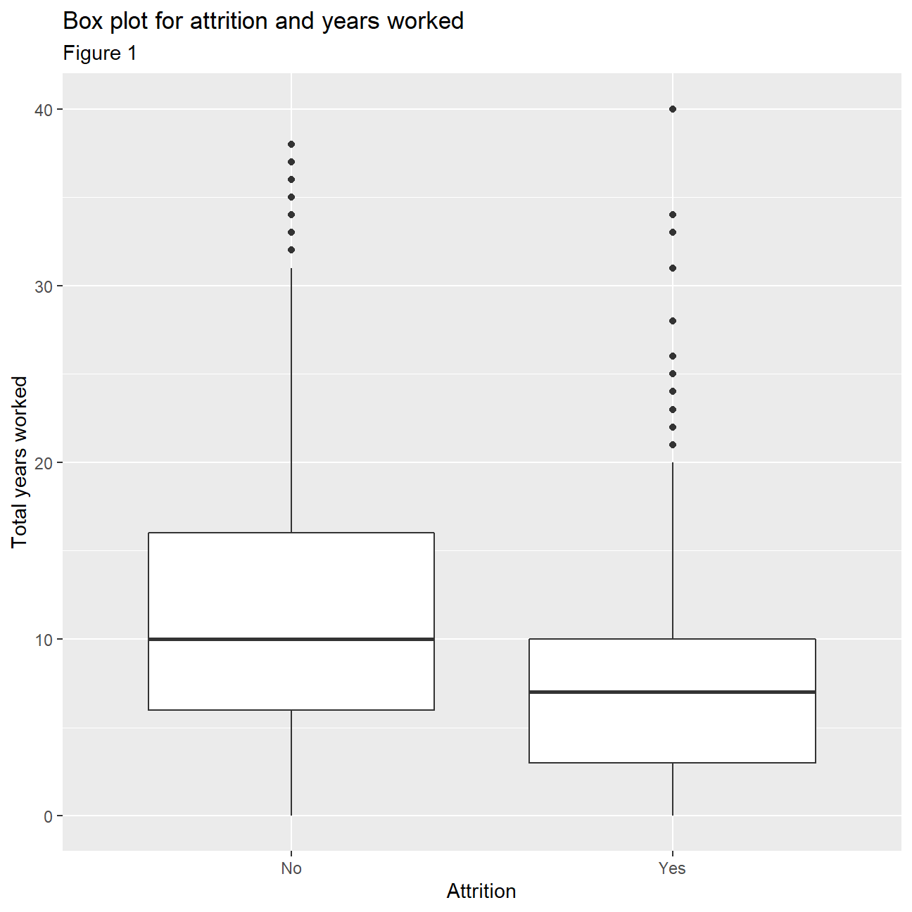
Firstly, we begin by looking at attrition rates in IBM. In Table 1 we can see that the company has an attrition rate of 16.1%. This means that 16.1 percent of the company’s listed employees left the company at the time the data set was created, which is not that high considering many young people may be using IBM as an opportunity to learn and then move into more senior positions at different companies. This can further be seen by drawing out a box plot comparing ‘attrition’ and the total number of years worked (Figure 1). From the box plots it is evident that it’s the people with less years of work that tend to leave the company. This however is only a hypothesis and needs some further analysis in order to be concluded with certainty.
Looking more closely at the distributions of some of the variables we can compare the mean and median in combination with 1st and 3rd quadrant, to make some inferences about normality and skewness. When the mean and median differ too much, there is a skewness and the distribution of the given variable is not normal. For example, age seems to be fairly normally distributed, even though the 1st and 3rd quadrant are not equally far away from the mean. Years at the company, years since last promotion and monthly income have some extreme outliers and differing median and mean making normality improbable. To confirm this, we plot density plots for each variable. It is clear that the variable that is closest to a normal distribution is ‘Age’ with the other three variables being heavily right skewed. From this, we can infer that employees across all ages can be found within IBM. At the same time there are extremely highly paid employees skewing the monthly income distribution and it is also evident that most employees are in the company for 0-10 years with only a few staying for longer periods of time.
An important area to explore is that of job satisfaction and work life balance in IBM. We can conclude that the majority of IBM employees seem to be happy with their job as from tables 3 and 4 we see that about 61.3% of employees report to have a Very High/High job satisfaction and a surprising 94.6% have at least a ‘Good’ work life balance. Only very few (5.4%) report a bad work life balance, however, 20% of employees are not satisfied with their job. This may be due to a number of different reasons such as income levels or hours worked, but it is always expected that some people will not be happy at their work and thus this percentage is not of major concern.
Next, we investigate how income levels compare to education. The box plots (figure 6) and histograms for education with monthly income (figure 10) indicate that more educated people tend to receive higher salaries. There are some outliers in all categories, except the ‘Doctor’ category. This indicates that we can find people from all academic backgrounds in senior, highly paid positions. Moreover, the distributions seem to be mostly skewed for the majority of education levels especially for employees with a Bachelors degree. Furthermore, plotting a bar chart (figure 9) of average incomes with education the conclusion that more educated people receive higher incomes is further supported. It is worth noting, however, that there is a big increase in average income for employees holding a ‘Doctorate’ where as for the rest of the education levels the increase in incomes is more gradual as education increases.
When looking at the box plots for monthly income with gender, (figure 7) interestingly enough, it seems that incomes are distributed quite similarly across genders with similar spread of values and medians of approximately 5000 dollars. This means that there is no gender income gap in IBM. Female employees even have a higher 25th and 75th percentile and slightly higher median, implying they receive slightly higher salaries.This is a very positive find as it shows that modern companies like IBM are promoting gender equality.
It is clear that income levels vary greatly between Job roles. From the box plots in figure 8 we can see that the highest paid positions are the ‘Managers’ and ‘Research Directors’ with respective medians of about 17 500 and 16 000 dollars. The spread of incomes for these two roles appear much higher than the rest. The job with the lowest pay is that of a ‘Sales Representative’ with income levels being very tightly spread around 2000-3000 dollars.
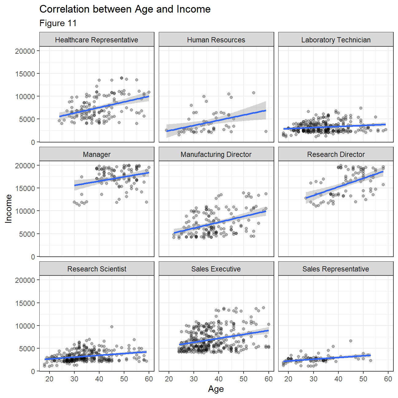
Lastly, we wanted to investigate how income varies with age across different job roles. From the plots in figure 11, we can see that for many jobs employees seem to be getting similar incomes across all ages with slight increases as people get older for some positions. For positions such as Healthcare representatives and Research Directors this phenomenon is more evident. This is quite interesting as usually we expect that older people are associated with more experience and thus higher pay but this is not the case for all positions here. We should note however that for the highest paid jobs of ‘Manager’ and ‘Research Director’ there are no 20-30 year olds employed so in general it is older people that work in the highest paid positions.
- How often do people leave the company (
attrition)
Table 1
hr_attrition_summarized <- hr_cleaned %>%
  count(attrition)

hr_attrition_summarized$percentage <- hr_attrition_summarized$n/sum(hr_attrition_summarized$n)

hr_attrition_summarized
## # A tibble: 2 x 3
## attrition n percentage
## <chr> <int> <dbl>
## 1 No 1233 0.839
## 2 Yes 237 0.161ggplot(hr_cleaned,aes(x=attrition,y=total_working_years))+
geom_boxplot()+
labs(
title="Box plot for attrition and years worked",
subtitle= "Figure 1",
x="Attrition",
y="Total years worked"
)
NULL## NULL- How are
age,years_at_company,monthly_incomeandyears_since_last_promotiondistributed? can you roughly guess which of these variables is closer to Normal just by looking at summary statistics?
Table 2
hr_cleaned %>%
  select(c("age", "years_at_company", "monthly_income",
           "years_since_last_promotion"))%>%
  summary()
## age years_at_company monthly_income years_since_last_promotion
## Min. :18.0 Min. : 0 Min. : 1009 Min. : 0.00
## 1st Qu.:30.0 1st Qu.: 3 1st Qu.: 2911 1st Qu.: 0.00
## Median :36.0 Median : 5 Median : 4919 Median : 1.00
## Mean :36.9 Mean : 7 Mean : 6503 Mean : 2.19
## 3rd Qu.:43.0 3rd Qu.: 9 3rd Qu.: 8379 3rd Qu.: 3.00
## Max. :60.0 Max. :40 Max. :19999 Max. :15.00hr_cleaned %>%
ggplot(aes(x=age))+
geom_density()+
theme_bw()+
labs(
title="Density Plot for Age",
subtitle= "Figure 2",
x="Age",
y="Density"
)+
NULL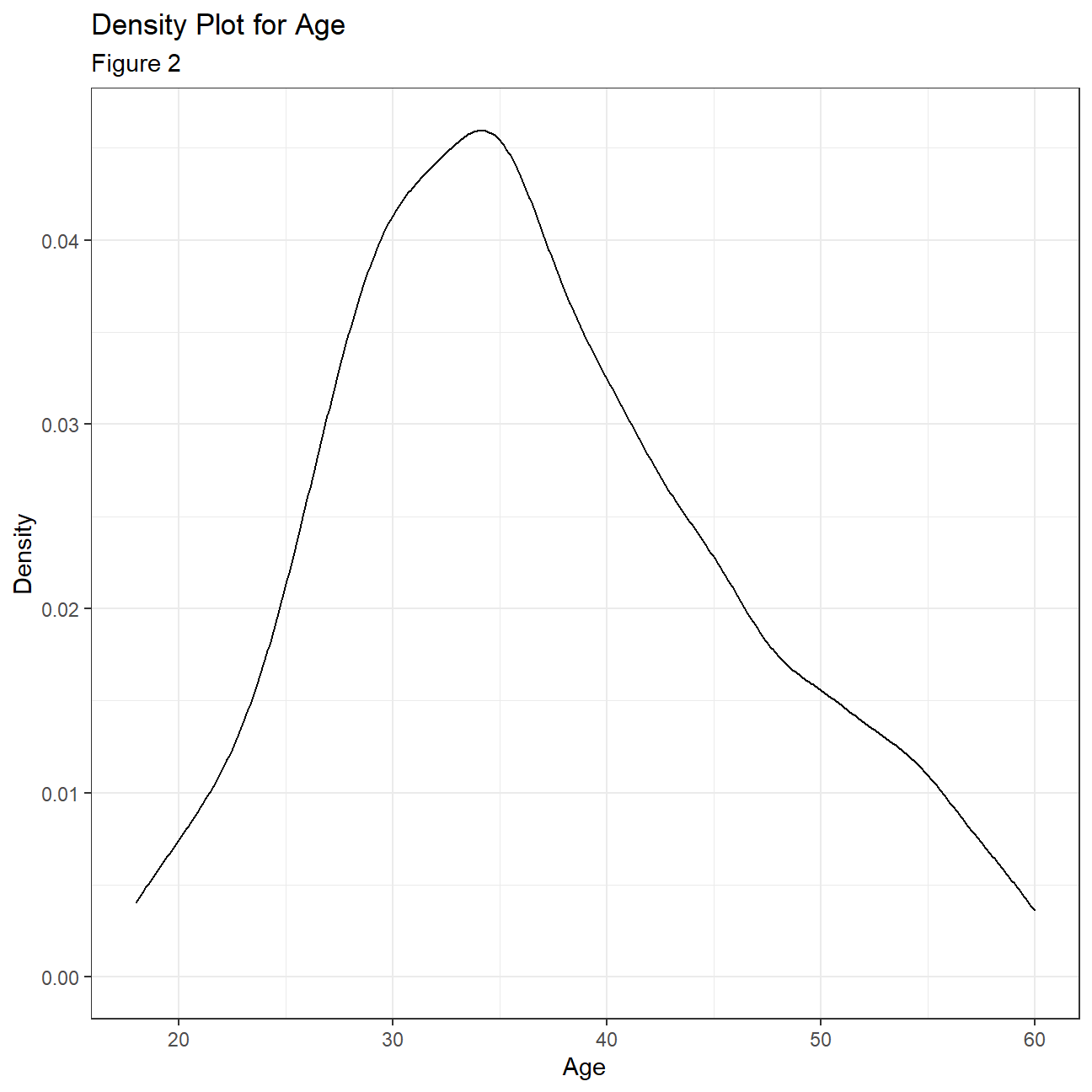
hr_cleaned %>%
  ggplot(aes(x=years_at_company))+
  geom_density()+
  theme_bw()+
  labs(
    title="Density Plot for Years at the company",
    subtitle= "Figure 3",
    x="Years at the company",
    y="Density"
  )+
  NULL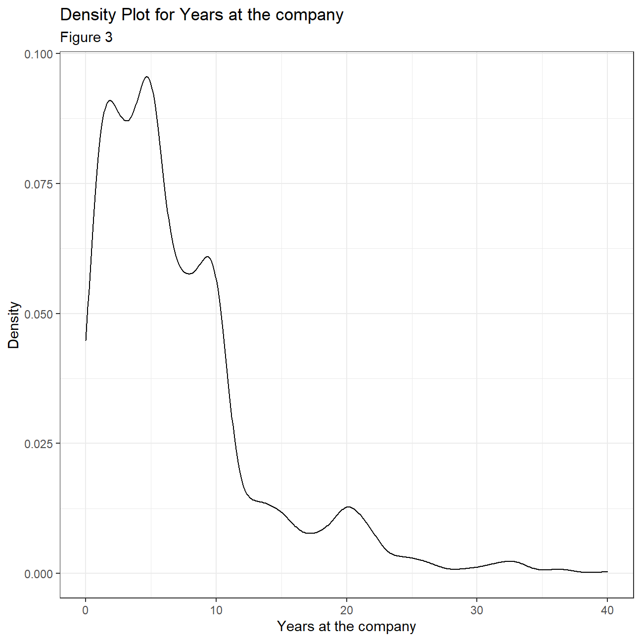
hr_cleaned %>%
  ggplot(aes(x=monthly_income))+
  geom_density()+
  theme_bw()+
  labs(
    title="Density Plot for Monthly income",
    subtitle= "Figure 4",
    x="Monthly Income",
    y="Density"
  )+
  NULL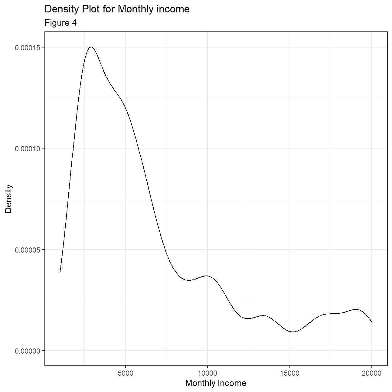
hr_cleaned %>%
  ggplot(aes(x=years_since_last_promotion))+
  geom_density()+
  theme_bw()+
  labs(
    title="Density Plot for Years since last promotion",
    subtitle= "Figure 5",
    x="Years since last promotion",
    y="Density"
  )+
  NULL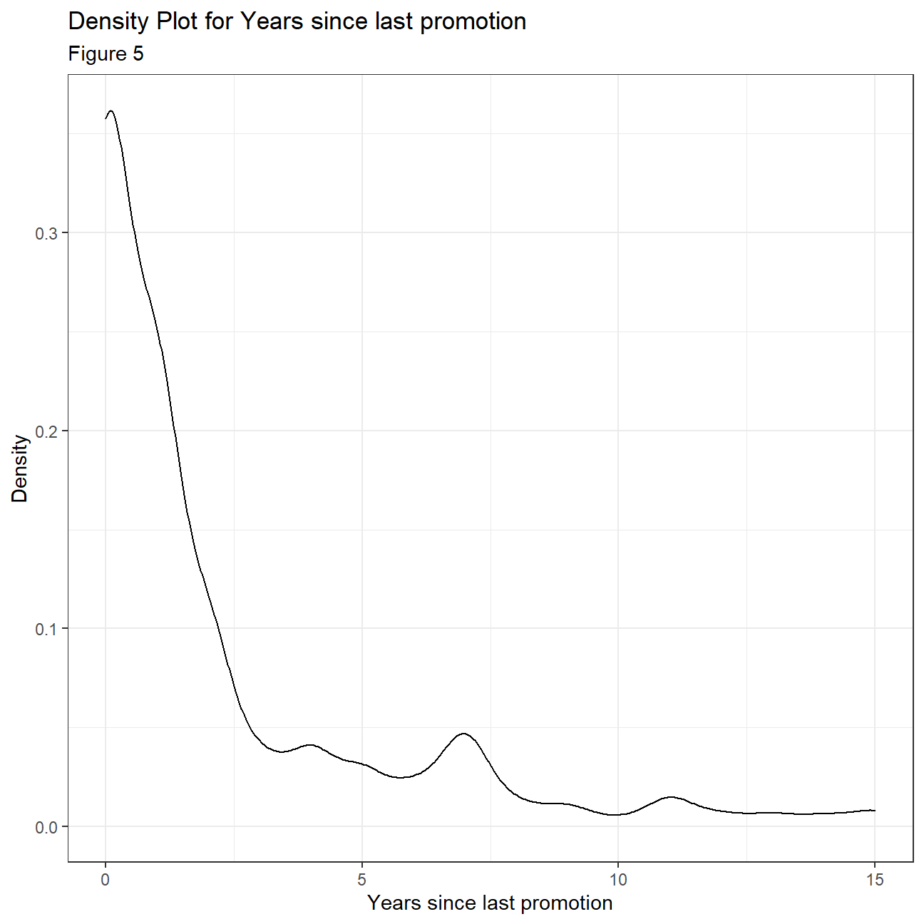
- How are
job_satisfactionandwork_life_balancedistributed? Don’t just report counts, but express categories as % of total
Table 3
hr_jobsatisfaction <- hr_cleaned %>%
  count(job_satisfaction)
hr_jobsatisfaction$percentage <- (hr_jobsatisfaction$n/sum(hr_jobsatisfaction$n)*100)
hr_jobsatisfaction
## # A tibble: 4 x 3
## job_satisfaction n percentage
## <chr> <int> <dbl>
## 1 High 442 30.1
## 2 Low 289 19.7
## 3 Medium 280 19.0
## 4 Very High 459 31.2Table 4
hr_worklbal <- hr_cleaned %>%
  count(work_life_balance)
hr_worklbal$percentage <- (hr_worklbal$n/sum(hr_worklbal$n))*100
hr_worklbal
## # A tibble: 4 x 3
## work_life_balance n percentage
## <chr> <int> <dbl>
## 1 Bad 80 5.44
## 2 Best 153 10.4
## 3 Better 893 60.7
## 4 Good 344 23.4- Is there any relationship between monthly income and education? Monthly income and gender?
Table 5
hr_income_education <- hr_cleaned %>%
  group_by(education) %>%
  summarize(
    avg_income = mean(monthly_income)
  )

hr_income_education
## # A tibble: 5 x 2
## education avg_income
## <chr> <dbl>
## 1 Bachelor 6517.
## 2 Below College 5641.
## 3 College 6227.
## 4 Doctor 8278.
## 5 Master 6832.ggplot(hr_cleaned, aes(x=reorder(education,monthly_income), y=monthly_income))+
geom_boxplot()+
labs(
title="Boxplot of Monthly income according to education",
subtitle= "Figure 6",
x="Education",
y="Income"
)+
NULL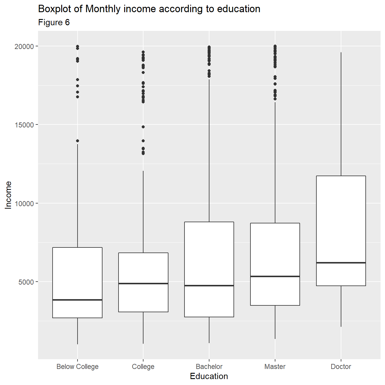
Table 6
hr_income_gender <- hr_cleaned %>%
  group_by(gender) %>%
  summarize(
    avg_income = mean(monthly_income)
  )

hr_income_gender
## # A tibble: 2 x 2
## gender avg_income
## <chr> <dbl>
## 1 Female 6687.
## 2 Male 6381.ggplot(hr_cleaned, aes(x=gender,y= monthly_income))+
geom_boxplot()+
labs(
title="Boxplot of Monthly income according to gender",
subtitle= "Figure 7",
x="Gender",
y="Income"
)+
NULL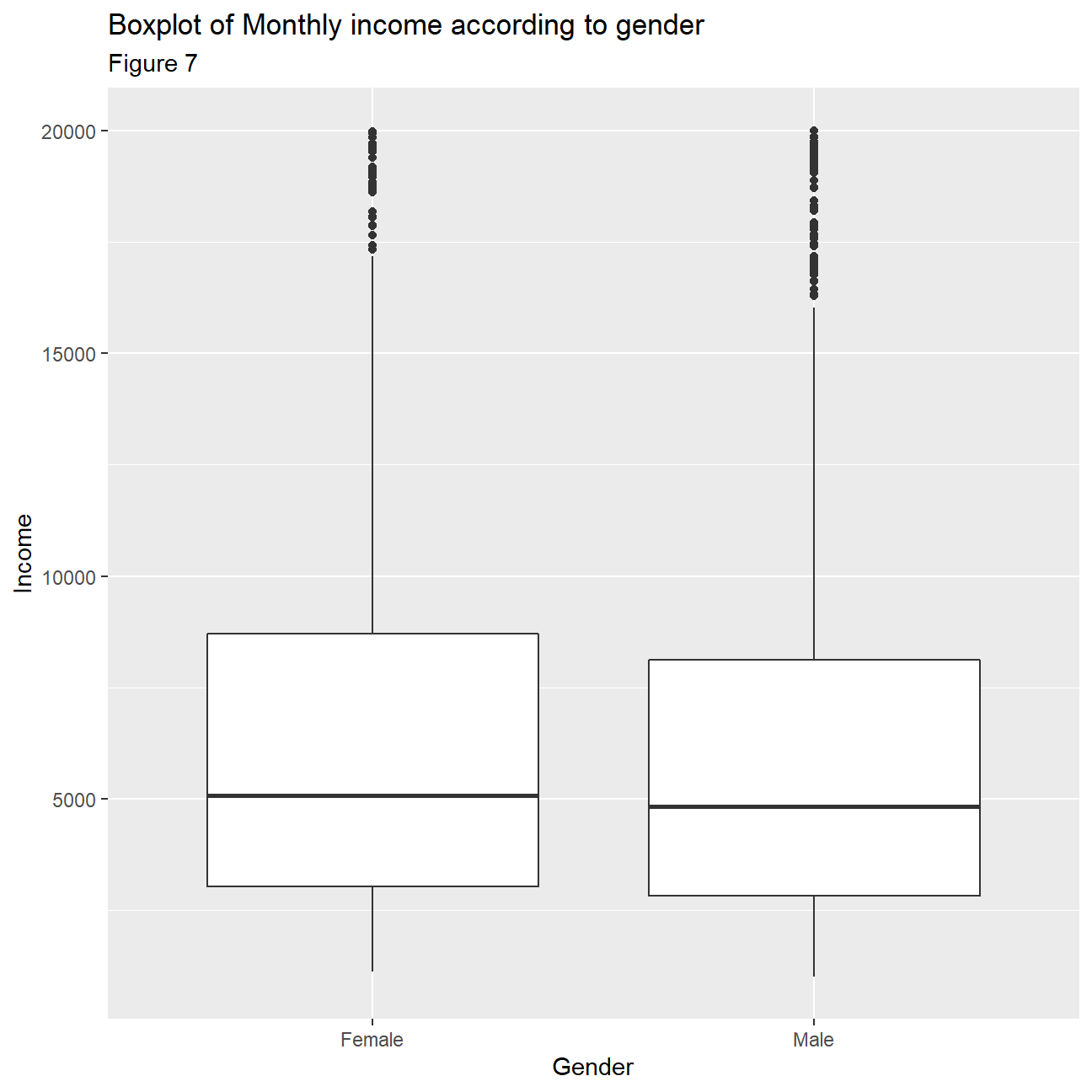
- Plot a boxplot of income vs job role. Make sure the highest-paid job roles appear first
ggplot(hr_cleaned, aes(x=reorder(job_role,-monthly_income), y=monthly_income))+
         geom_boxplot()+
  labs(
    title="Job Role vs. Income",
    subtitle= "Figure 8",
    x="Job Role",
    y="Income"
  )+
  theme(axis.text.x = element_text(angle=90, vjust=0.5, hjust=1))+
  NULL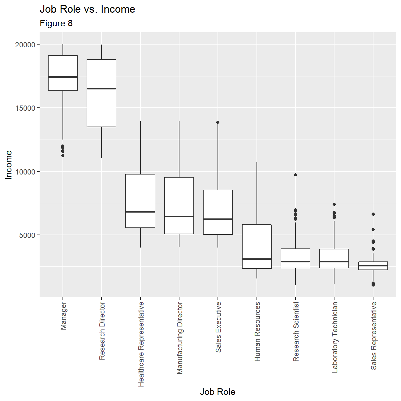
- Calculate and plot a bar chart of the mean (or median?) income by education level.
hr_mean_income_education <- hr_cleaned %>%
  group_by(education) %>%
  summarize(
    mean_income=mean(monthly_income),
    median_income=median(monthly_income)
    )

ggplot(hr_mean_income_education,aes(x=reorder(education, -mean_income),
                                    y=mean_income))+
  geom_col()+
  labs(
    title="Average Income according to Education Level",
    subtitle= "Figure 9",
    x="Education Level",
    y="Average income"
    )+
  NULL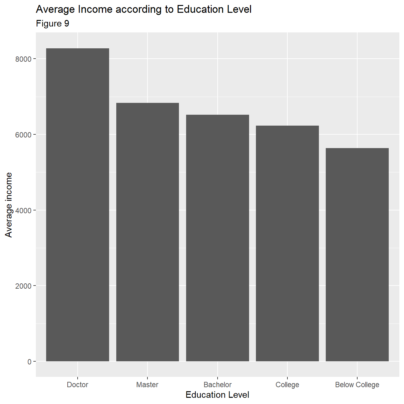
- Plot the distribution of income by education level. Use a facet_wrap and a theme from
ggthemes
ggplot(hr_cleaned,aes(x=monthly_income))+
  geom_histogram()+
  facet_wrap(~education)+
  theme_wsj()+
  theme(plot.title = element_text(size=15),
        plot.subtitle = element_text(size=12),
        axis.text.x = element_text(angle=45, size = 10, vjust=0.5, hjust=1),
        axis.text.y = element_text(angle=45, size = 10, vjust=0.5, hjust=1))+
  labs(
    title="Distribution of Income by Education Level",
    subtitle= "Figure 10",
    x="Income",
    y="Count"
  )+

  NULL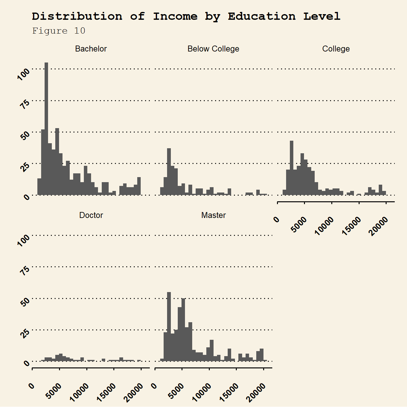
- Plot income vs age, faceted by
job_role
ggplot(hr_cleaned, aes(x=age, y=monthly_income))+
  geom_point(alpha=0.3)+
  geom_smooth(method = "lm")+
  theme_bw()+
  labs(
    title="Correlation between Age and Income",
    subtitle= "Figure 11",
    x="Age",
    y="Income"
  )+
  facet_wrap(~job_role)+
  NULL