Pre-programme Assignment

Task 1: gapminder country comparison
glimpse(gapminder)## Rows: 1,704
## Columns: 6
## $ country <fct> "Afghanistan", "Afghanistan", "Afghanistan", "Afghanistan", ~
## $ continent <fct> Asia, Asia, Asia, Asia, Asia, Asia, Asia, Asia, Asia, Asia, ~
## $ year <int> 1952, 1957, 1962, 1967, 1972, 1977, 1982, 1987, 1992, 1997, ~
## $ lifeExp <dbl> 28.801, 30.332, 31.997, 34.020, 36.088, 38.438, 39.854, 40.8~
## $ pop <int> 8425333, 9240934, 10267083, 11537966, 13079460, 14880372, 12~
## $ gdpPercap <dbl> 779.4453, 820.8530, 853.1007, 836.1971, 739.9811, 786.1134, ~head(gapminder, 20) ## # A tibble: 20 x 6
## country continent year lifeExp pop gdpPercap
## <fct> <fct> <int> <dbl> <int> <dbl>
## 1 Afghanistan Asia 1952 28.8 8425333 779.
## 2 Afghanistan Asia 1957 30.3 9240934 821.
## 3 Afghanistan Asia 1962 32.0 10267083 853.
## 4 Afghanistan Asia 1967 34.0 11537966 836.
## 5 Afghanistan Asia 1972 36.1 13079460 740.
## 6 Afghanistan Asia 1977 38.4 14880372 786.
## 7 Afghanistan Asia 1982 39.9 12881816 978.
## 8 Afghanistan Asia 1987 40.8 13867957 852.
## 9 Afghanistan Asia 1992 41.7 16317921 649.
## 10 Afghanistan Asia 1997 41.8 22227415 635.
## 11 Afghanistan Asia 2002 42.1 25268405 727.
## 12 Afghanistan Asia 2007 43.8 31889923 975.
## 13 Albania Europe 1952 55.2 1282697 1601.
## 14 Albania Europe 1957 59.3 1476505 1942.
## 15 Albania Europe 1962 64.8 1728137 2313.
## 16 Albania Europe 1967 66.2 1984060 2760.
## 17 Albania Europe 1972 67.7 2263554 3313.
## 18 Albania Europe 1977 68.9 2509048 3533.
## 19 Albania Europe 1982 70.4 2780097 3631.
## 20 Albania Europe 1987 72 3075321 3739.country_data <- gapminder %>%
filter(country == "China")
continent_data <- gapminder %>%
filter(continent == "Asia")plot1 <- ggplot(data = country_data, mapping = aes(x = year, y = lifeExp))+
geom_point() +
geom_smooth(se = FALSE)+
NULL
plot1## `geom_smooth()` using method = 'loess' and formula 'y ~ x'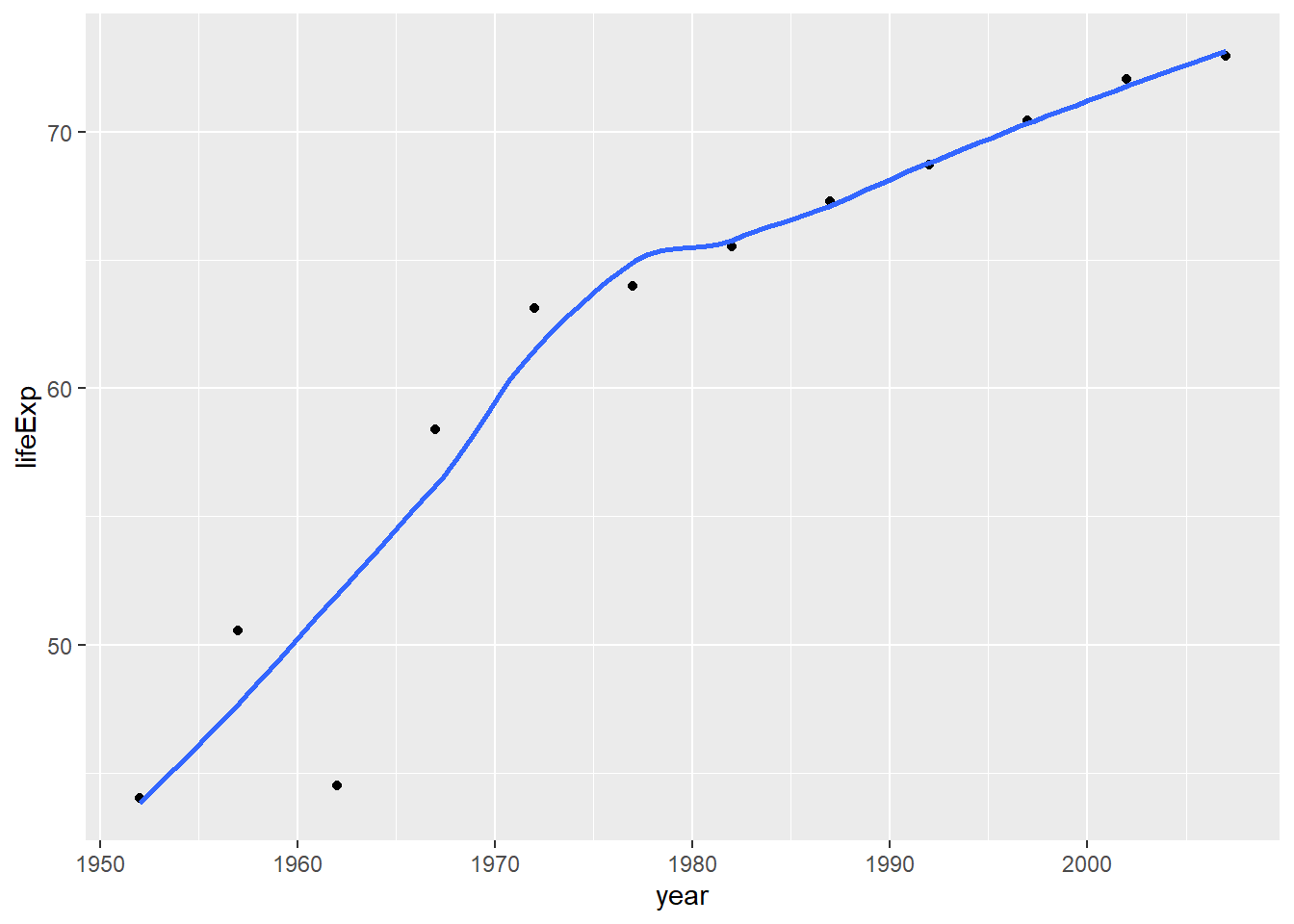
plot1<- plot1 +
  labs(title = "How life expectancy has changed over the years for China ",
      x = "Year ",
      y = "Life Expectancy ") +
  NULL


plot1
## `geom_smooth()` using method = 'loess' and formula 'y ~ x'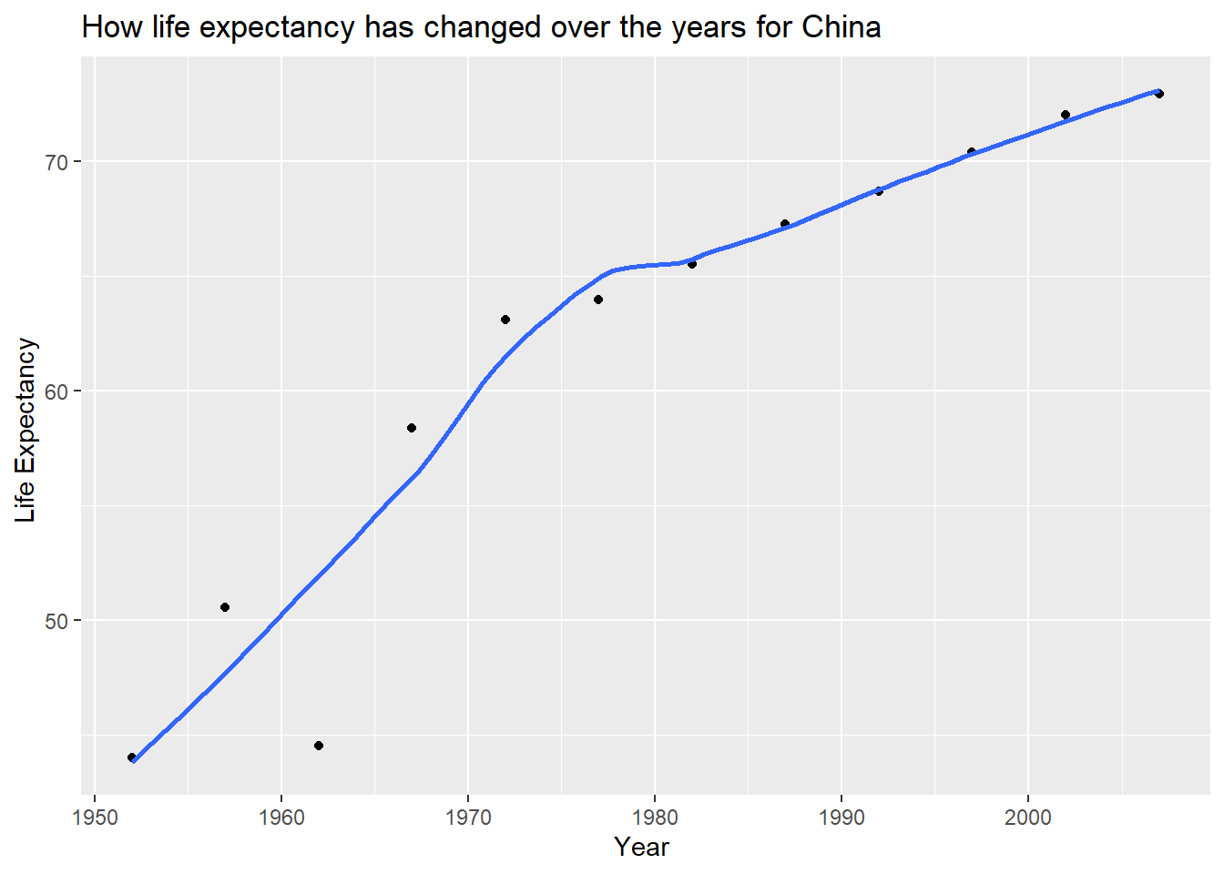
ggplot(data = continent_data, mapping = aes(x = year , y = lifeExp , colour= country, group = country))+
  geom_point() +
  geom_smooth(se = FALSE) +
  NULL
## `geom_smooth()` using method = 'loess' and formula 'y ~ x'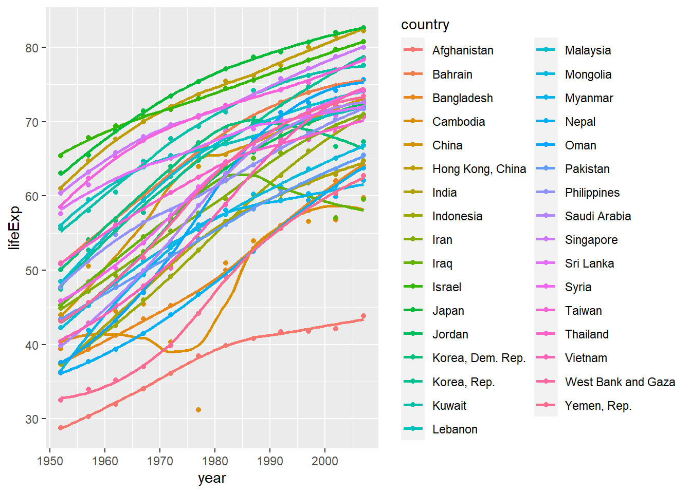
ggplot(data = gapminder , mapping = aes(x = year , y = lifeExp , colour= continent))+
  geom_point() +
  geom_smooth(se = FALSE) +
  facet_wrap(~continent) +
  theme(legend.position="none") +
  NULL
## `geom_smooth()` using method = 'loess' and formula 'y ~ x'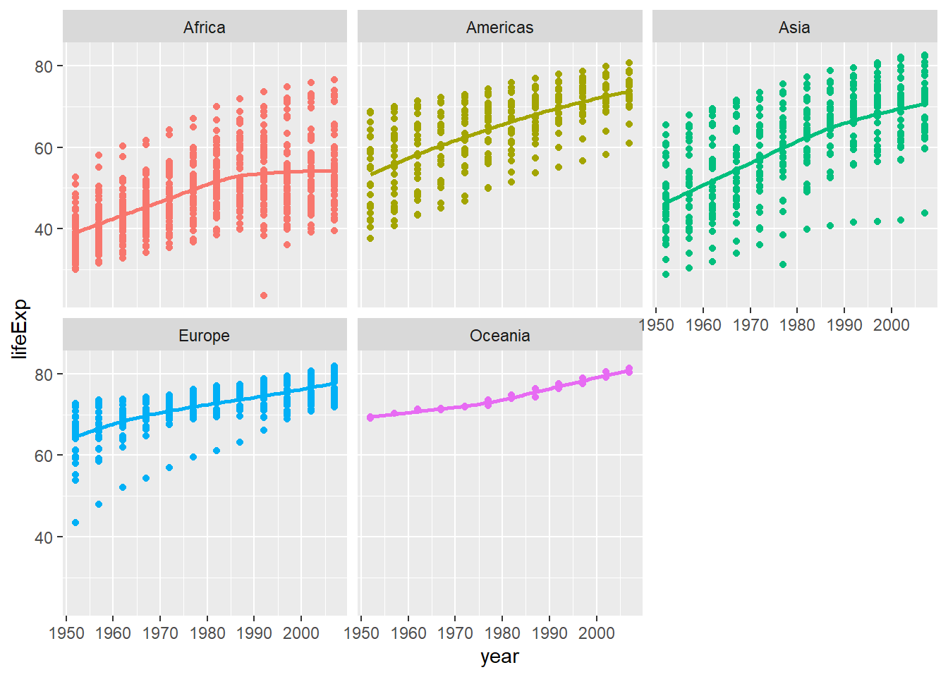
Type your answer after this blockquote. - All continents show increasing trends in life expectancy, with Africa showing the slowest increase and Asiz showing the fastest increase. - Life expectancy growth slows in Asia and Africa. - Overall, Life expectancy is highest in Europe and lowest in Africa.
Task 2: Brexit vote analysis
brexit_results <- read_csv(here::here("data","brexit_results.csv"))


glimpse(brexit_results)
## Rows: 632
## Columns: 11
## $ Seat <chr> "Aldershot", "Aldridge-Brownhills", "Altrincham and Sale W~
## $ con_2015 <dbl> 50.592, 52.050, 52.994, 43.979, 60.788, 22.418, 52.454, 22~
## $ lab_2015 <dbl> 18.333, 22.369, 26.686, 34.781, 11.197, 41.022, 18.441, 49~
## $ ld_2015 <dbl> 8.824, 3.367, 8.383, 2.975, 7.192, 14.828, 5.984, 2.423, 1~
## $ ukip_2015 <dbl> 17.867, 19.624, 8.011, 15.887, 14.438, 21.409, 18.821, 21.~
## $ leave_share <dbl> 57.89777, 67.79635, 38.58780, 65.29912, 49.70111, 70.47289~
## $ born_in_uk <dbl> 83.10464, 96.12207, 90.48566, 97.30437, 93.33793, 96.96214~
## $ male <dbl> 49.89896, 48.92951, 48.90621, 49.21657, 48.00189, 49.17185~
## $ unemployed <dbl> 3.637000, 4.553607, 3.039963, 4.261173, 2.468100, 4.742731~
## $ degree <dbl> 13.870661, 9.974114, 28.600135, 9.336294, 18.775591, 6.085~
## $ age_18to24 <dbl> 9.406093, 7.325850, 6.437453, 7.747801, 5.734730, 8.209863~# histogram
ggplot(brexit_results, aes(x = leave_share)) +
geom_histogram(binwidth = 2.5)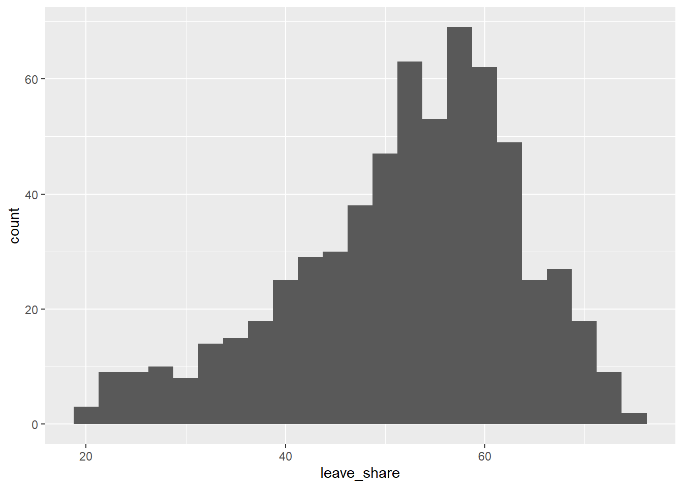
# density plot-- think smoothed histogram
ggplot(brexit_results, aes(x = leave_share)) +
  geom_density()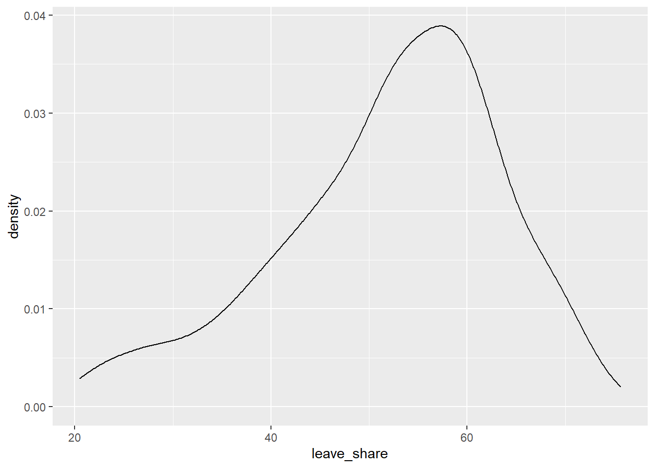
# The empirical cumulative distribution function (ECDF)
ggplot(brexit_results, aes(x = leave_share)) +
  stat_ecdf(geom = "step", pad = FALSE) +
  scale_y_continuous(labels = scales::percent)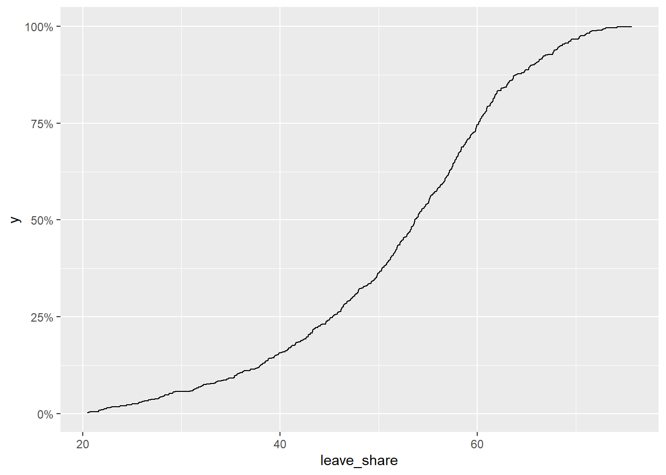
brexit_results %>%
  select(leave_share, born_in_uk) %>%
  cor()
## leave_share born_in_uk
## leave_share 1.0000000 0.4934295
## born_in_uk 0.4934295 1.0000000ggplot(brexit_results, aes(x = born_in_uk, y = leave_share)) +
geom_point(alpha=0.3) +
# add a smoothing line, and use method="lm" to get the best straight-line
geom_smooth(method = "lm") +
# use a white background and frame the plot with a black box
theme_bw() +
NULL## `geom_smooth()` using formula 'y ~ x'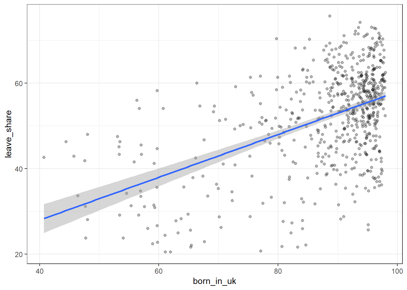
Type your answer after, and outside, this blockquote. - Slightly more than half of the Constituencies support Britain leaving the EU. - Higher rates of being born in the UK are more likely to support Brexit. - The higher the rate of birth in the UK, the smaller the range of the percent of supporting for Brexit
Task 3: Animal rescue incidents attended by the London Fire Brigade
url <- "https://data.london.gov.uk/download/animal-rescue-incidents-attended-by-lfb/8a7d91c2-9aec-4bde-937a-3998f4717cd8/Animal%20Rescue%20incidents%20attended%20by%20LFB%20from%20Jan%202009.csv"

animal_rescue <- read_csv(url,
                          locale = locale(encoding = "CP1252")) %>%
  janitor::clean_names()


glimpse(animal_rescue)
## Rows: 7,772
## Columns: 31
## $ incident_number <chr> "139091", "275091", "2075091", "2872091"~
## $ date_time_of_call <chr> "01/01/2009 03:01", "01/01/2009 08:51", ~
## $ cal_year <dbl> 2009, 2009, 2009, 2009, 2009, 2009, 2009~
## $ fin_year <chr> "2008/09", "2008/09", "2008/09", "2008/0~
## $ type_of_incident <chr> "Special Service", "Special Service", "S~
## $ pump_count <chr> "1", "1", "1", "1", "1", "1", "1", "1", ~
## $ pump_hours_total <chr> "2", "1", "1", "1", "1", "1", "1", "1", ~
## $ hourly_notional_cost <dbl> 255, 255, 255, 255, 255, 255, 255, 255, ~
## $ incident_notional_cost <chr> "510", "255", "255", "255", "255", "255"~
## $ final_description <chr> "Redacted", "Redacted", "Redacted", "Red~
## $ animal_group_parent <chr> "Dog", "Fox", "Dog", "Horse", "Rabbit", ~
## $ originof_call <chr> "Person (land line)", "Person (land line~
## $ property_type <chr> "House - single occupancy", "Railings", ~
## $ property_category <chr> "Dwelling", "Outdoor Structure", "Outdoo~
## $ special_service_type_category <chr> "Other animal assistance", "Other animal~
## $ special_service_type <chr> "Animal assistance involving livestock -~
## $ ward_code <chr> "E05011467", "E05000169", "E05000558", "~
## $ ward <chr> "Crystal Palace & Upper Norwood", "Woods~
## $ borough_code <chr> "E09000008", "E09000008", "E09000029", "~
## $ borough <chr> "Croydon", "Croydon", "Sutton", "Hilling~
## $ stn_ground_name <chr> "Norbury", "Woodside", "Wallington", "Ru~
## $ uprn <chr> "NULL", "NULL", "NULL", "100021491149", ~
## $ street <chr> "Waddington Way", "Grasmere Road", "Mill~
## $ usrn <chr> "20500146", "NULL", "NULL", "21401484", ~
## $ postcode_district <chr> "SE19", "SE25", "SM5", "UB9", "RM3", "RM~
## $ easting_m <chr> "NULL", "534785", "528041", "504689", "N~
## $ northing_m <chr> "NULL", "167546", "164923", "190685", "N~
## $ easting_rounded <dbl> 532350, 534750, 528050, 504650, 554650, ~
## $ northing_rounded <dbl> 170050, 167550, 164950, 190650, 192350, ~
## $ latitude <chr> "NULL", "51.39095371", "51.36894086", "5~
## $ longitude <chr> "NULL", "-0.064166887", "-0.161985191", ~animal_rescue %>%
dplyr::group_by(cal_year) %>%
summarise(count=n())## # A tibble: 13 x 2
## cal_year count
## <dbl> <int>
## 1 2009 568
## 2 2010 611
## 3 2011 620
## 4 2012 603
## 5 2013 585
## 6 2014 583
## 7 2015 540
## 8 2016 604
## 9 2017 539
## 10 2018 610
## 11 2019 604
## 12 2020 758
## 13 2021 547animal_rescue %>%
count(cal_year, name="count")## # A tibble: 13 x 2
## cal_year count
## <dbl> <int>
## 1 2009 568
## 2 2010 611
## 3 2011 620
## 4 2012 603
## 5 2013 585
## 6 2014 583
## 7 2015 540
## 8 2016 604
## 9 2017 539
## 10 2018 610
## 11 2019 604
## 12 2020 758
## 13 2021 547animal_rescue %>%
group_by(animal_group_parent) %>%
#group_by and summarise will produce a new column with the count in each animal group
summarise(count = n()) %>%
# mutate adds a new column; here we calculate the percentage
mutate(percent = round(100*count/sum(count),2)) %>%
# arrange() sorts the data by percent. Since the default sorting is min to max and we would like to see it sorted
# in descending order (max to min), we use arrange(desc())
arrange(desc(percent))## # A tibble: 28 x 3
## animal_group_parent count percent
## <chr> <int> <dbl>
## 1 Cat 3736 48.1
## 2 Bird 1611 20.7
## 3 Dog 1213 15.6
## 4 Fox 366 4.71
## 5 Unknown - Domestic Animal Or Pet 199 2.56
## 6 Horse 195 2.51
## 7 Deer 132 1.7
## 8 Unknown - Wild Animal 93 1.2
## 9 Squirrel 66 0.85
## 10 Unknown - Heavy Livestock Animal 50 0.64
## # ... with 18 more rowsanimal_rescue %>%
#count does the same thing as group_by and summarise
# name = "count" will call the column with the counts "count" ( exciting, I know)
# and 'sort=TRUE' will sort them from max to min
count(animal_group_parent, name="count", sort=TRUE) %>%
mutate(percent = round(100*count/sum(count),2))## # A tibble: 28 x 3
## animal_group_parent count percent
## <chr> <int> <dbl>
## 1 Cat 3736 48.1
## 2 Bird 1611 20.7
## 3 Dog 1213 15.6
## 4 Fox 366 4.71
## 5 Unknown - Domestic Animal Or Pet 199 2.56
## 6 Horse 195 2.51
## 7 Deer 132 1.7
## 8 Unknown - Wild Animal 93 1.2
## 9 Squirrel 66 0.85
## 10 Unknown - Heavy Livestock Animal 50 0.64
## # ... with 18 more rows# what type is variable incident_notional_cost from dataframe `animal_rescue`
typeof(animal_rescue$incident_notional_cost)## [1] "character"# readr::parse_number() will convert any numerical values stored as characters into numbers
animal_rescue <- animal_rescue %>%
# we use mutate() to use the parse_number() function and overwrite the same variable
mutate(incident_notional_cost = parse_number(incident_notional_cost))
# incident_notional_cost from dataframe `animal_rescue` is now 'double' or numeric
typeof(animal_rescue$incident_notional_cost)## [1] "double"animal_rescue %>%
# group by animal_group_parent
group_by(animal_group_parent) %>%
# filter resulting data, so each group has at least 6 observations
filter(n()>6) %>%
# summarise() will collapse all values into 3 values: the mean, median, and count
# we use na.rm=TRUE to make sure we remove any NAs, or cases where we do not have the incident cos
summarise(mean_incident_cost = mean (incident_notional_cost, na.rm=TRUE),
median_incident_cost = median (incident_notional_cost, na.rm=TRUE),
sd_incident_cost = sd (incident_notional_cost, na.rm=TRUE),
min_incident_cost = min (incident_notional_cost, na.rm=TRUE),
max_incident_cost = max (incident_notional_cost, na.rm=TRUE),
count = n()) %>%
# sort the resulting data in descending order. You choose whether to sort by count or mean cost.
arrange(desc(count))## # A tibble: 16 x 7
## animal_group_parent mean_incident_co~ median_incident_~ sd_incident_cost
## <chr> <dbl> <dbl> <dbl>
## 1 Cat 343. 298 160.
## 2 Bird 344. 328 135.
## 3 Dog 347. 298 169.
## 4 Fox 373. 328 206.
## 5 Unknown - Domestic Anim~ 326. 295 117.
## 6 Horse 740. 596 541.
## 7 Deer 417. 333 286.
## 8 Unknown - Wild Animal 416. 333 324.
## 9 Squirrel 313. 326 57.1
## 10 Unknown - Heavy Livesto~ 374. 260 263.
## 11 cat 324. 290 94.1
## 12 Hamster 315. 290 95.0
## 13 Snake 356. 339 105.
## 14 Rabbit 309. 326 32.2
## 15 Ferret 309. 333 39.4
## 16 Cow 634. 520 475.
## # ... with 3 more variables: min_incident_cost <dbl>, max_incident_cost <dbl>,
## # count <int># base_plot
base_plot <- animal_rescue %>%
group_by(animal_group_parent) %>%
filter(n()>6) %>%
ggplot(aes(x=incident_notional_cost))+
facet_wrap(~animal_group_parent, scales = "free")+
theme_bw()
base_plot + geom_histogram()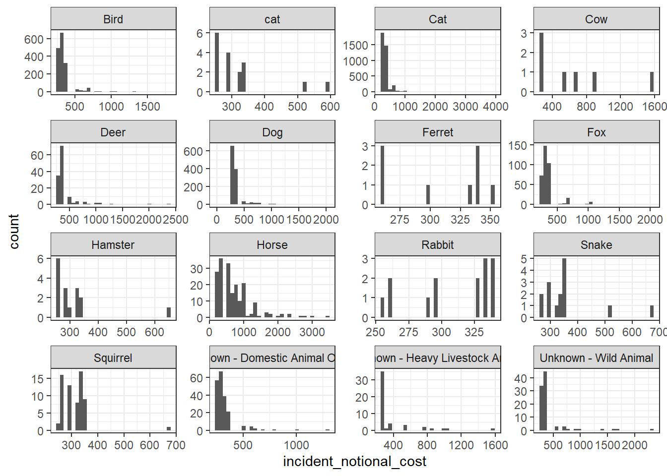
base_plot + geom_density()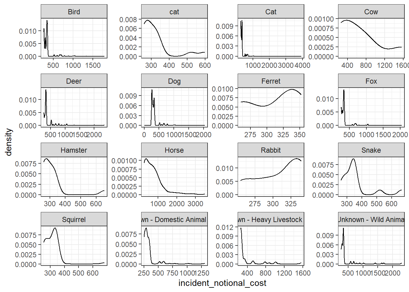
base_plot + geom_boxplot()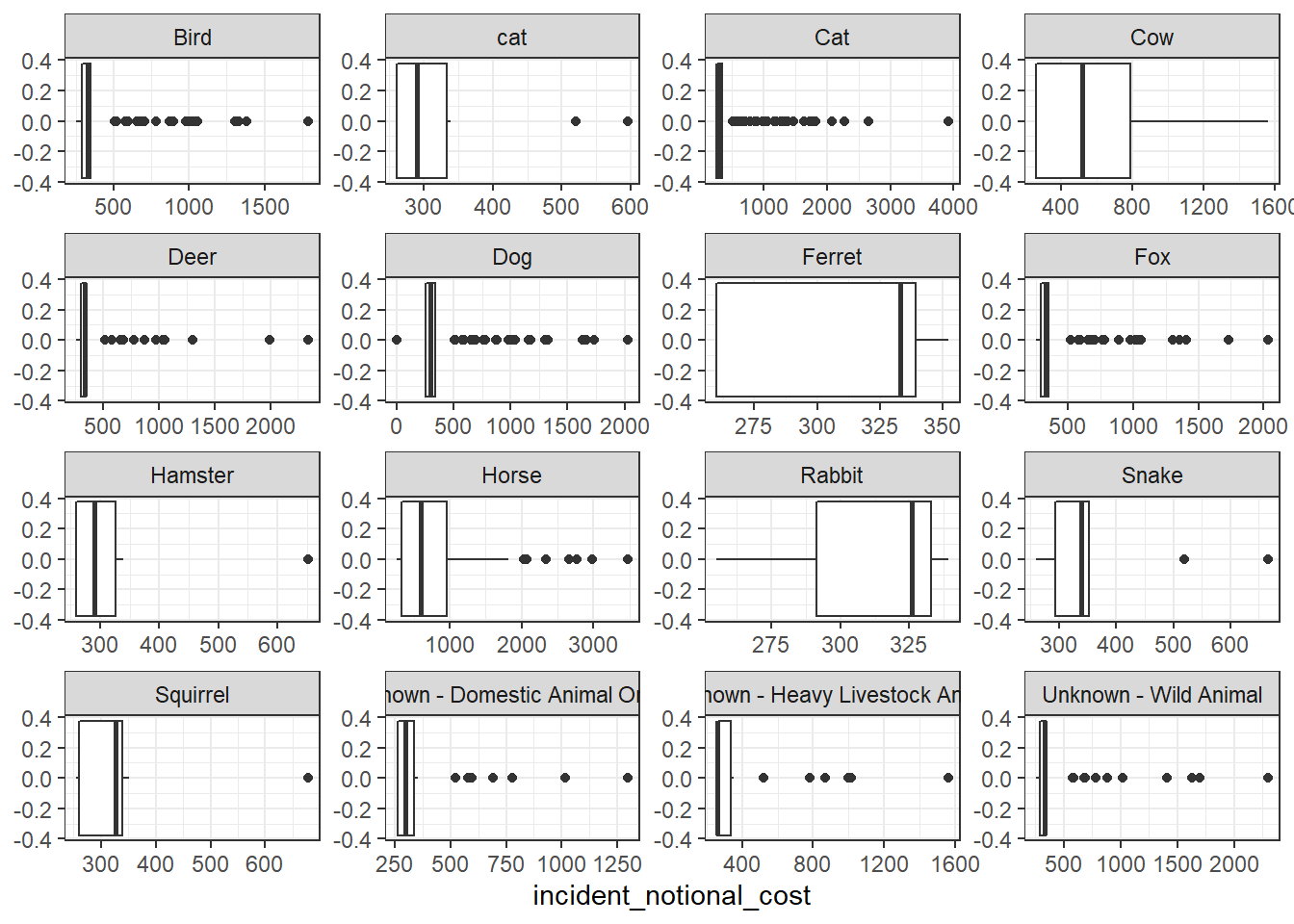
base_plot + stat_ecdf(geom = "step", pad = FALSE) +
  scale_y_continuous(labels = scales::percent)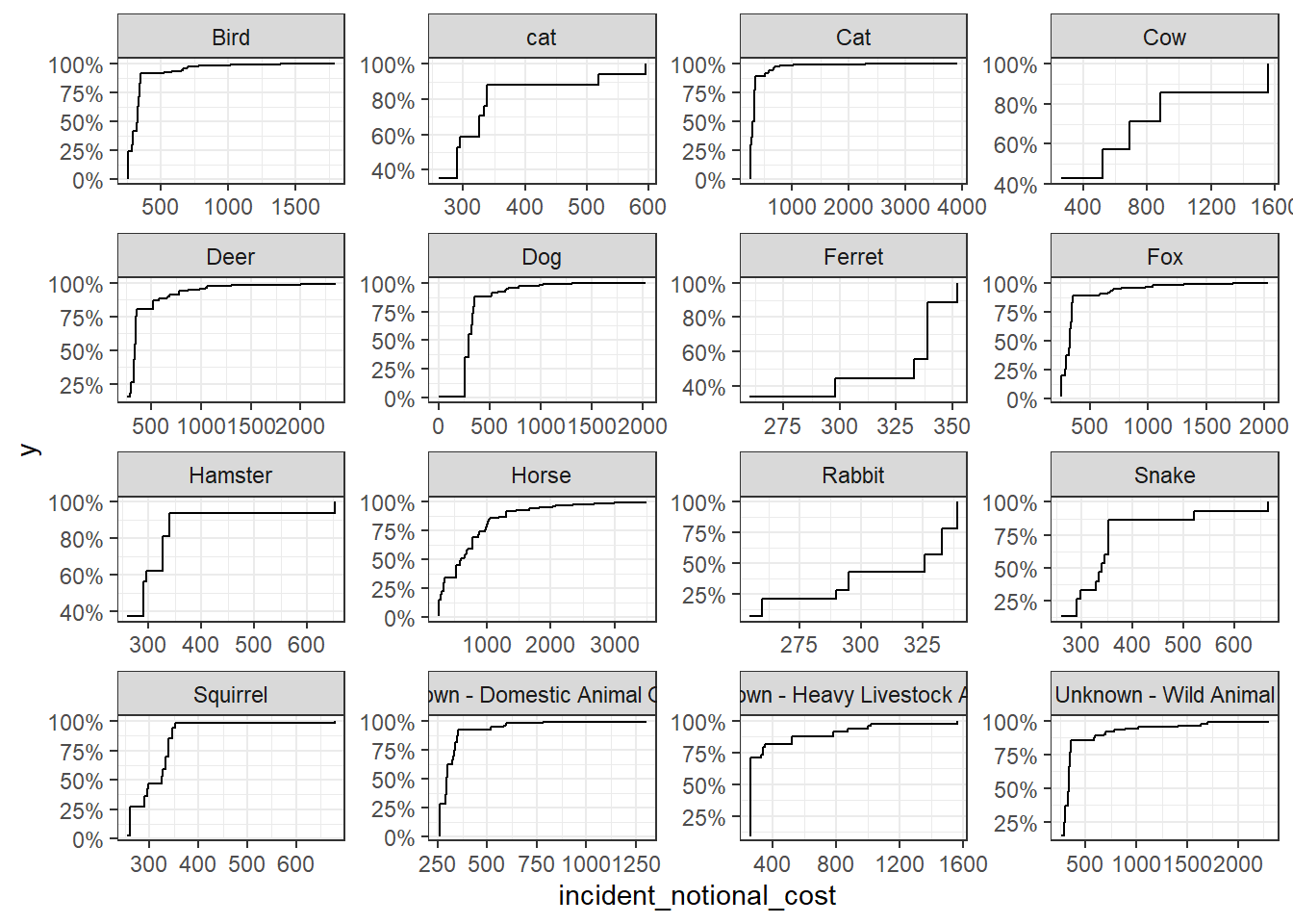
- The third one (boxplot) communicates the variability of the
incident_notional_costvalues best. - Horse and Cow are more expensive.